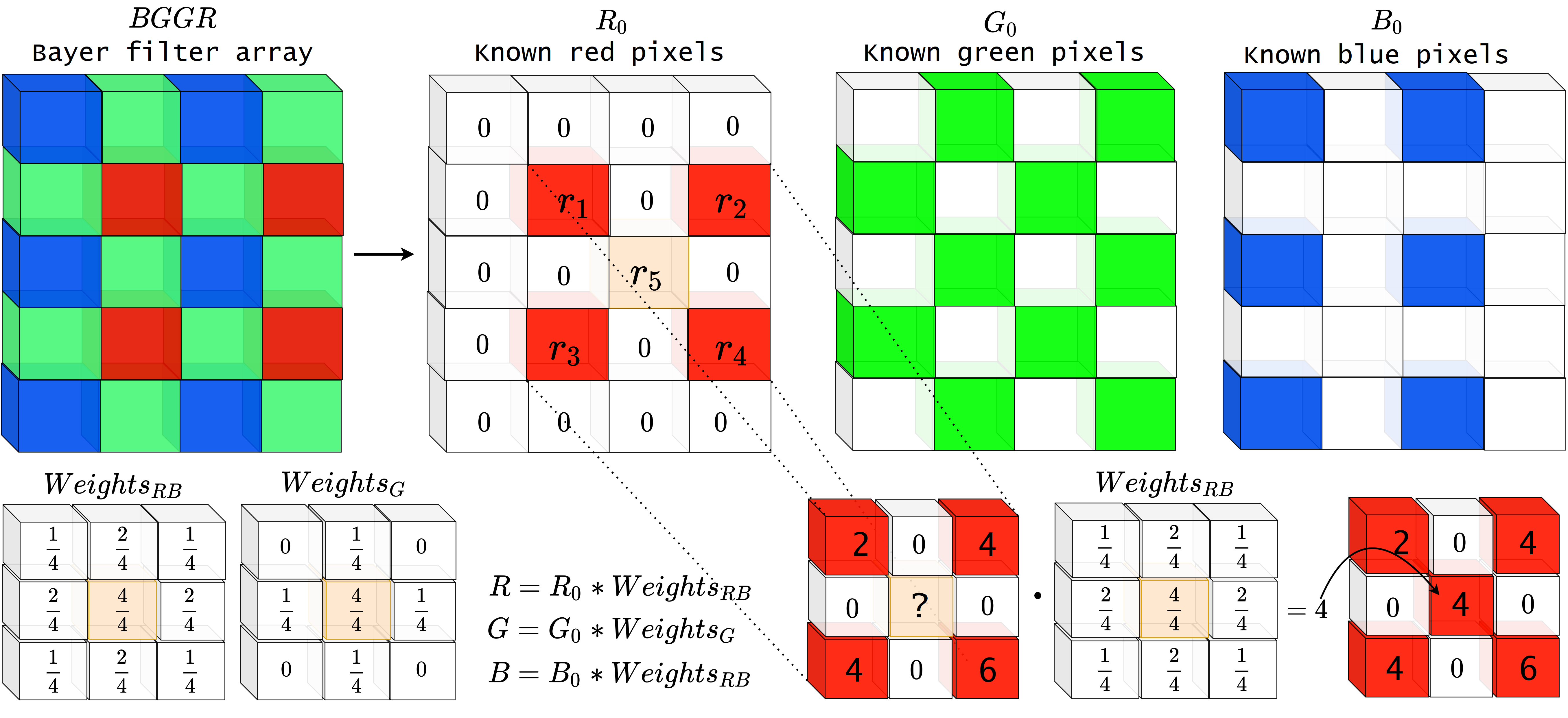
2.4 How to pre-process a color filter array?

As we learned, a colour sensor provides colour filter arrays (CFAs), which need to be pre-processed in order to achieve an RGB image. Convolution and bilinear interpolation is one simple, but efficient combination of methods.

Figure 1 shows that there are missing values in each RGB colour frame. However, the value of each missing pixel can be easily calculated, for example, with a bilinear interpolation, where each of the 2D plane’s pixel values is an average of the neighbouring pixels. The red, green and blue planes can be calculated separately with convolutional operations by placing zeros to missing values in R0, G0 and B0, and sliding a weighted 3 × 3 kernel over the red, green and blue colour planes, filling the middle pixel with the result (Eskelinen, 2019).

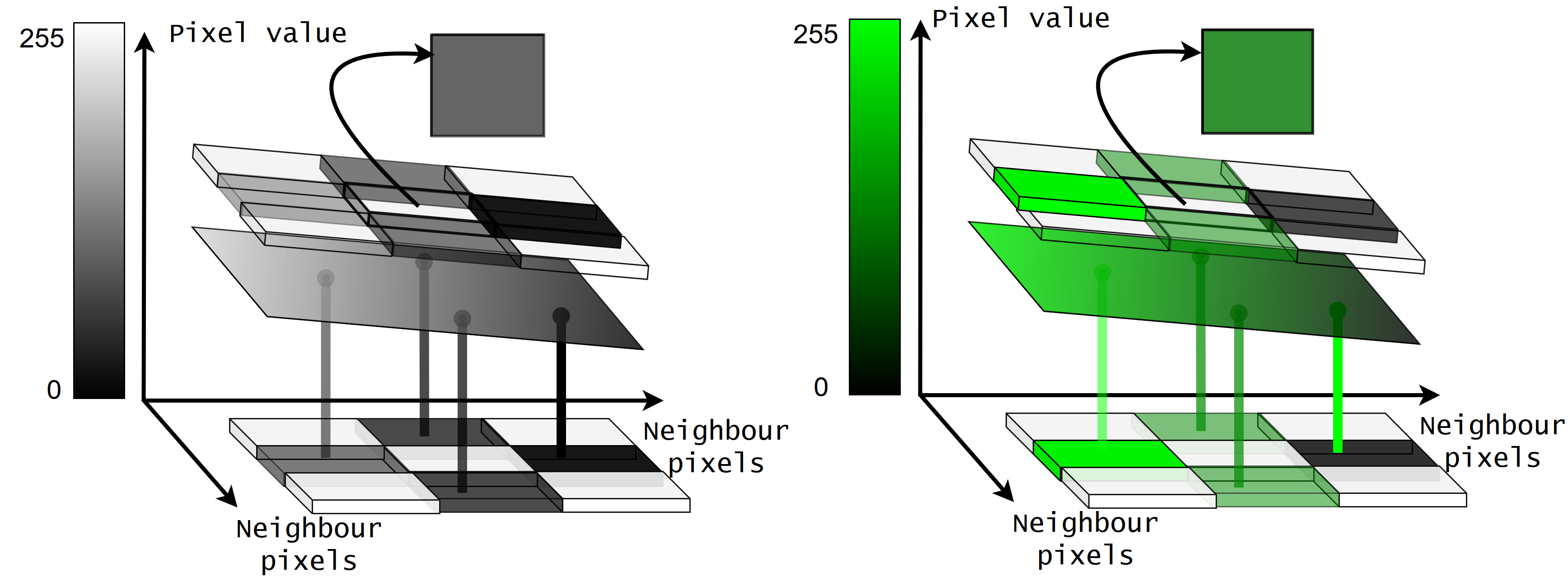
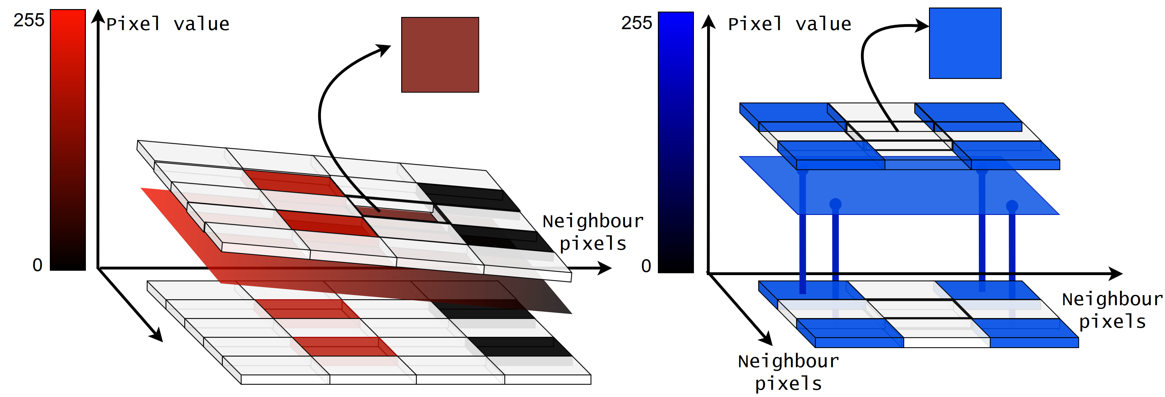
Figure 1. Bilinear convolution. The Bayer BGGR colour filter array is divided into three colour planes R0, G0 and B0. Each of the missing values is set to zero (0). A weighted kernel (WeightsRG or WeightsG) slides over each pixel of the colour planes (y and x directions). The value of the middle pixel is the weighted average of the neighbouring pixels.

Below, Figure 2 illustrates how the behaviour of the pixel values in the RGB colourspace. The minimum RGB value of one channel is zero (0), which is visualised as black. The highest value 255, is white in a greyscale image, but in a colour channel, it is visualised as the most intensive red, green or blue tone. Intuitively the interpolation can be seen as a pixel value surface formed from the mean of neighbouring pixels. The pixel value surface is drawn above the original Bayer pattern in the illustration (Figure 2). After interpolation, the top pattern with the individual middle pixel represents the computed pixel value. The green and red examples are fading colours, so the surfaces are inclined. The blue represents an equally intensive pixel neighbourhood, where the pixel value surface is drawn horizontally straight.

FIGURE 2 Bilinear interpolation. Intuitively, the bilinear interpolation can be seen as linear towards the image’s x and y directions, where the mean of the neighbouring pixels forms a surface, where the middle pixel gets its pixel colour value. The colour bar represents the RGB colours’ minimum and maximum values (0 to 255). A pixel captured with a high number of photons reaches higher values, resulting in a “bright colour”. A pixel with a low number of photons gets values close to zero, and the pixel is seen as black.

Found something useful? Wish to cite? This post is based on my dissertation. For citations and more information, click here to see the scientific version of it.

References

Eskelinen, M. 2019. Computational methods for hyperspectral imaging using Fabry-Perot interferometers and colour cameras. URL:http://urn.fi/URN:ISBN:978-951-39-7967-6.