If you wish to test your idea of target-wisely customised imager, it can be built combining a machine vision sensor with optical or optomechanical components. There exists various of components to choose from.
Extension tubes (Figure 1) are useful for creating more complex prototype imagers than a basic sensor and a lens. With extension tubes, the optomechanical components can be mounted together.
Figure 1. C- mount extension tube
Different band-pass filters (Figure 2), beam splitters (Figure 3) and lenses can be used to produce, for instance, a simple two-channel spectral imager.
Figure 2. Series of band-pass filters, FWHM 10 nm. These filters vary between 380 -700nm.
Figure 3. This beam splitter divides the incoming light 50:50 to two sensors. This way, we can create a MV system that captures the target scene at the same time with two cameras. The sensors can be different, and we can use different filters to gain more detailed information from the target.
While designing such a system, it is valuable to understand that the system’s parameters will change depending on where the extension is added. For example, suppose the extension is placed between the lens and the sensor. In that case, the image-side focal length increases, decreasing the minimal working distance and field of view, magnifying the object (Greivenkamp 2004).
Examples in the future posts
As an example of special imager, a spectral camera typically consists of an optomechanical components, lenses and a sensor. The optomechanical component can be a prism or mechanical, dispersing the incoming light to wavelengths. We will later discuss over the spectral imagers and spend some time getting known with the dispersive components and their operating principles.
Focal length (FL) affects the field of view and magnification, as it is one of the most important parameters when choosing optics.
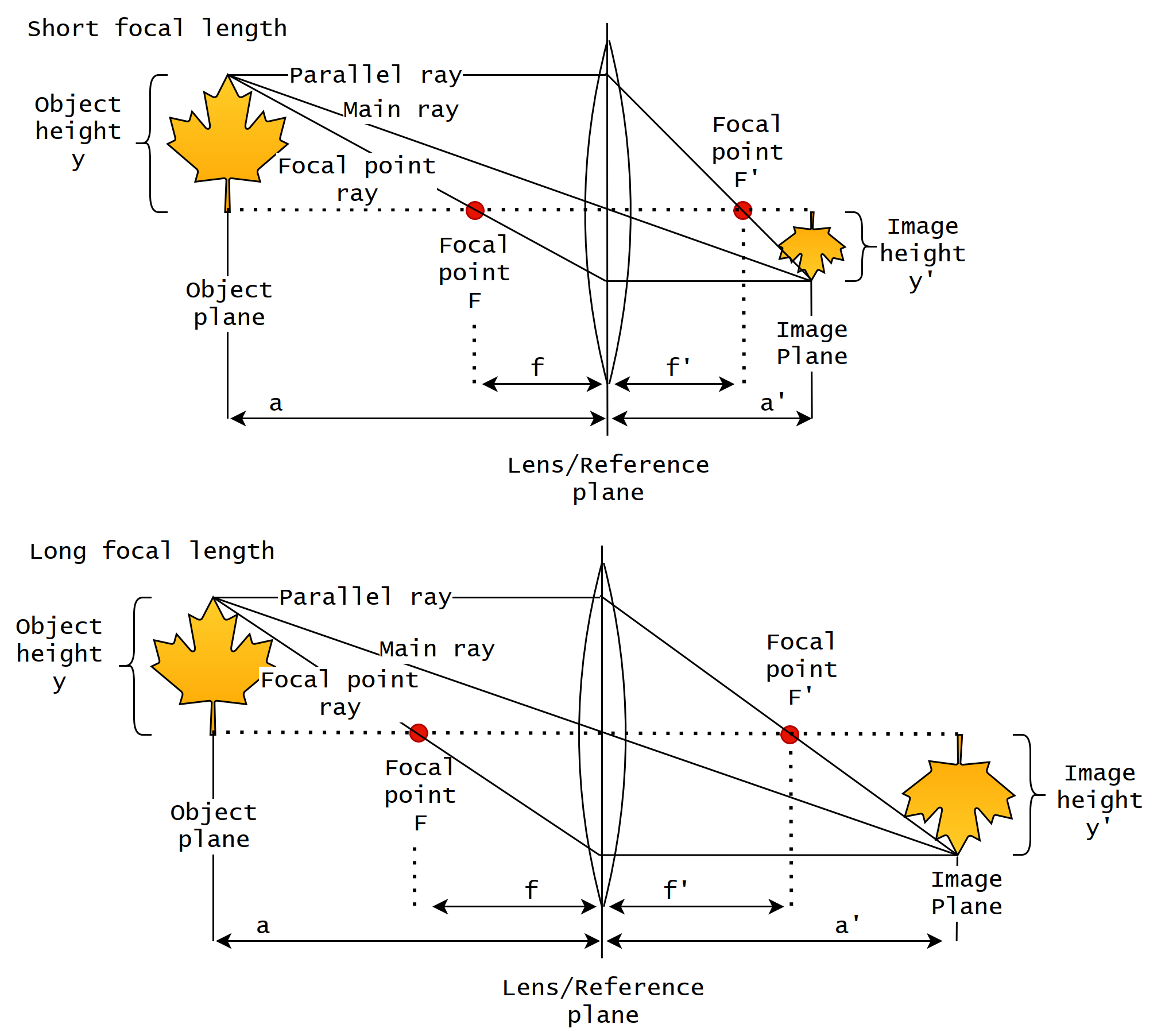
Focal length refers to the distance between the main plane of the lens and a particular point where the light is focused from infinity. Below, Figure 1 visualises how the focal length, marked with f and f ′, affects the image height. A long focal length magnifies more than a short one (Greivenkamp 2004).
FIGURE 1 Long and short focal length. Figure parameters: a: working distance, a′: image distance, f : object-side focal length, f ′: image-side focal length, F: object side focal point, F′: image side focal point, y: object height and y′ image height. Increased focal length magnifies the object size on image plane (y′), while the working distance can remain unchanged.
The working distance, object size and focal length affect the magnification. From above, Figure 15, we can see that a longer focal length increases the magnification without extending the working distance a. Magnification β can be approximated for a non-complex optical setups as follows (Greivenkamp 2004):
(1)
For thin lenses:
(2)
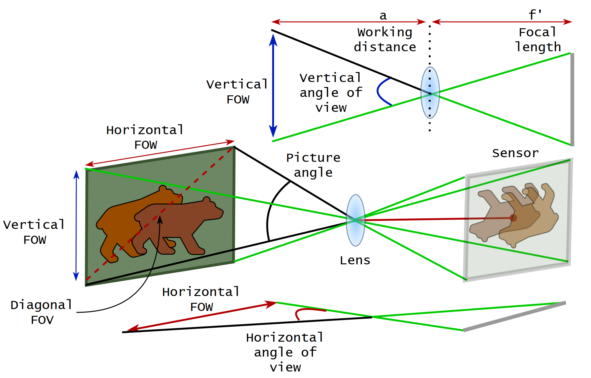
Below, Figure 2 explains the lens opening angles and their relations with the horizontal, vertical and diagonal field of view (FOV). By looking at the angles and rays of the image, we can see that the relation between the field of view and working distance correlates; the image field of view decreases while the working distance shortens and vice versa.
FIGURE 2 Field of view (FOW) is affected by the lens focal length, lens opening angles and working distance. These parameters can be evaluated, and the lens should be selected according to the working distance and target measures.
The relation between the opening angle and focal length is the opposite; the larger the focal length, the narrower the opening angle. Most of the lens parameters described in Table 2 (Post 3.1) can be calculated either with pen and paper or using services like Vision Doctor (Doctor 2022) or sensor manufacturers’ web tools, which are provided for designing imaging systems.
While there are many parameters to consider, the infrared (IR) cut and possible colour corrections are the least worth mentioning features. Suppose an imaging system is for spectral imaging, and the interesting wavelength range is in IR. It might be good to exclude lenses designed to block IR light or lenses that have some other undesirable colour corrections by default (Greivenkamp 2004; Stemmer 2022).
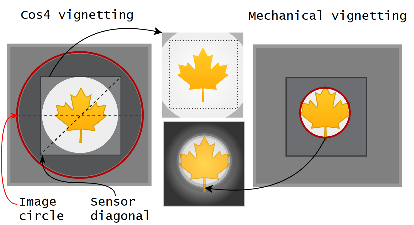
A carefully selected lens provides high-quality images from the objects. The image circle is formed when a light strikes a perpendicular target, i.e., the sensor, which forms a circle of light.
Below, Figure 1 shows the relation between the lens image circle and sensor diagonal. As a lens-related property, the image quality typically deteriorates towards border areas, and the images might suffer from shading or vignetting.
To avoid mechanical vignetting, choosing the right size optics with the sensor is necessary. If the lens image circle or lens mount is too small, the image will be heavily vignetted (lower-middle image).
Figure 1. Image vignetting and shading. In the illustration on the left, the image circle is larger than the sensor diagonal, and the shade is caused by Cos4 vignetting. In contrast, in the illustration on the right, the image circle is smaller than the sensor diagonal, causing mechanical vignetting. Both situations can cause vignetting or shades. If the object is in the middle of the non-shaded area, the image can be cropped, as shown with a dotted line in the upper-middle image. The right side example produces images that are not usable (lower-middle image).
Another source of vignetting, Cos4, is seen in the upper-middle image (above, Figure 1). If the light travels to the edges of the image from a further distance and reaches the sensor at an angle, it affects image quality; the light falloff is determined by the cos4(θ) function, where θ is the angle of incoming the light with respect to the image space’s optical axis.
The drop in intensity is more significant for wide incidence angles, causing the image to appear brighter at the centre and darker at the edges (Greivenkamp 2004). Since it is sometimes difficult to find inexpensive optics of the right size for the desired sensor (other parameters that depend on the target might limit the selection), the lens image circle can be oversized. In such cases, the images can be cropped and used, or the effect can be controlled by decreasing the aperture size.
Machine vision and computer vision terminology might be confusing. Here is a definition, that we will use in this website.
The first high-level term in this field was computer vision. Since the core of the 1970s intelligent robot was a vision, the research area was named after it (Ejiri 2007). In terms of research content, however, the case and name refer more to the current interpreter of machine vision.
According to Smith et al. (2021), the current de facto interpretation of machine vision is “computer vision techniques to help solve practical industrial problems that involve a significant visual component”. The state-of-the-art interpretation combines machine vision and deep learning methods and considers machine vision as one of the core technologies of artificial intelligence (Smith et al. 2021).
Figure 1. Relationship between artificial intelligence, machine learning and deep learning. Machine learning is a subset of artificial intelligence, and deep learning is a subset of particular machine learning.
Figure 2. Relationship between the terms machine vision, computer vision and machine learning. Machine vision has two sub-terms; computer vision and image capturing. The essence of computer vision lies in machine learning.